Für eine geschlossene Bearbeitung von Transformationsaufgaben ist von Nachteil, dass die Translation auf einer Addition und alle anderen Transformationen auf der Multiplikation von Matrizen beruhen. Durch das Hinzufügen einer weiteren, virtuellen Koordinate kann dieser Mangel behoben werden. Wird dies in geeigneter Weise getan (siehe Rändern, Abschnitt Rändern von Determinanten) bleibt der Wert der Matrix bekanntlich unverändert.
Am Beispiel der Translation wird dies deutlich:
\( P' = P + T = \left( {\begin{array}{cc}x\\y\end{array} } \right) + \left( {\begin{array}{cc}{ {t_x} }\\{ {t_y} }\end{array} } \right) \qquad \Rightarrow \qquad P' = \left( {\begin{array}{cc}1&0&{ {t_x} }\\0&1&{ {t_y} }\\0&0&1\end{array} } \right) \cdot \left( {\begin{array}{cc}x\\y\\1\end{array} } \right) \) Gl. 227
Wird das Matrixprodukt ausgeführt, entsteht exakt das Gleichungssystem von Gl. 216. Die letzte Zeile wird dabei unberücksichtigt gelassen.
\( P' = \left( {\begin{array}{cc}1&0&{ {t_x} }\\0&1&{ {t_y} }\\0&0&1\end{array} } \right) \cdot \left( {\begin{array}{cc}x\\y\\1\end{array} } \right) = \left( {\begin{array}{cc}{1 \cdot x + 0 \cdot y + {t_x} \cdot 1}\\{0 \cdot x + 1 \cdot y + {t_y} \cdot 1}\\{0 \cdot x + 0 \cdot y + 1 \cdot 1}\end{array} } \right) = \left( {\begin{array}{cc}{x + {t_x} }\\{y + {t_y} }\\1\end{array} } \right) \) Gl. 228
Alle anderen Transformationen werden nach dem gleichen Prinzip erweitert:
Skalierung:
\(P' = S \cdot P = \left( {\begin{array}{cc}{ {s_x} }&0&0\\0&{ {s_y} }&0\\0&0&1\end{array} } \right) \cdot \left( {\begin{array}{cc}x\\y\\1\end{array} } \right)\) Gl. 229
Scherung:
\(P' = Sh \cdot P = \left( {\begin{array}{cc}1&{ {a_x} }&0\\{ {a_y} }&1&0\\0&0&1\end{array} } \right) \cdot \left( {\begin{array}{cc}x\\y\\1\end{array} } \right)\) Gl. 230
Rotation:
\(P' = R \cdot P = \left( {\begin{array}{cc}{\cos \phi }&{ - \sin \phi }&0\\{\sin \phi }&{\cos \phi }&0\\0&0&1\end{array} } \right) \cdot \left( {\begin{array}{cc}x\\y\\1\end{array} } \right)\) Gl. 231
Ein weiterer Vorteil der homogenen Matrizen liegt darin, dass alle multiplikativ verknüpften Transformationen, bevor die eigentliche Multiplikation mit dem Punktvektor erfolgt, vorbereitend ausgeführt werden können. Damit wird sehr viel Rechenaufwand und Zeit gespart, wenn viele Punkte auf die gleiche Weise transformiert werden sollen.
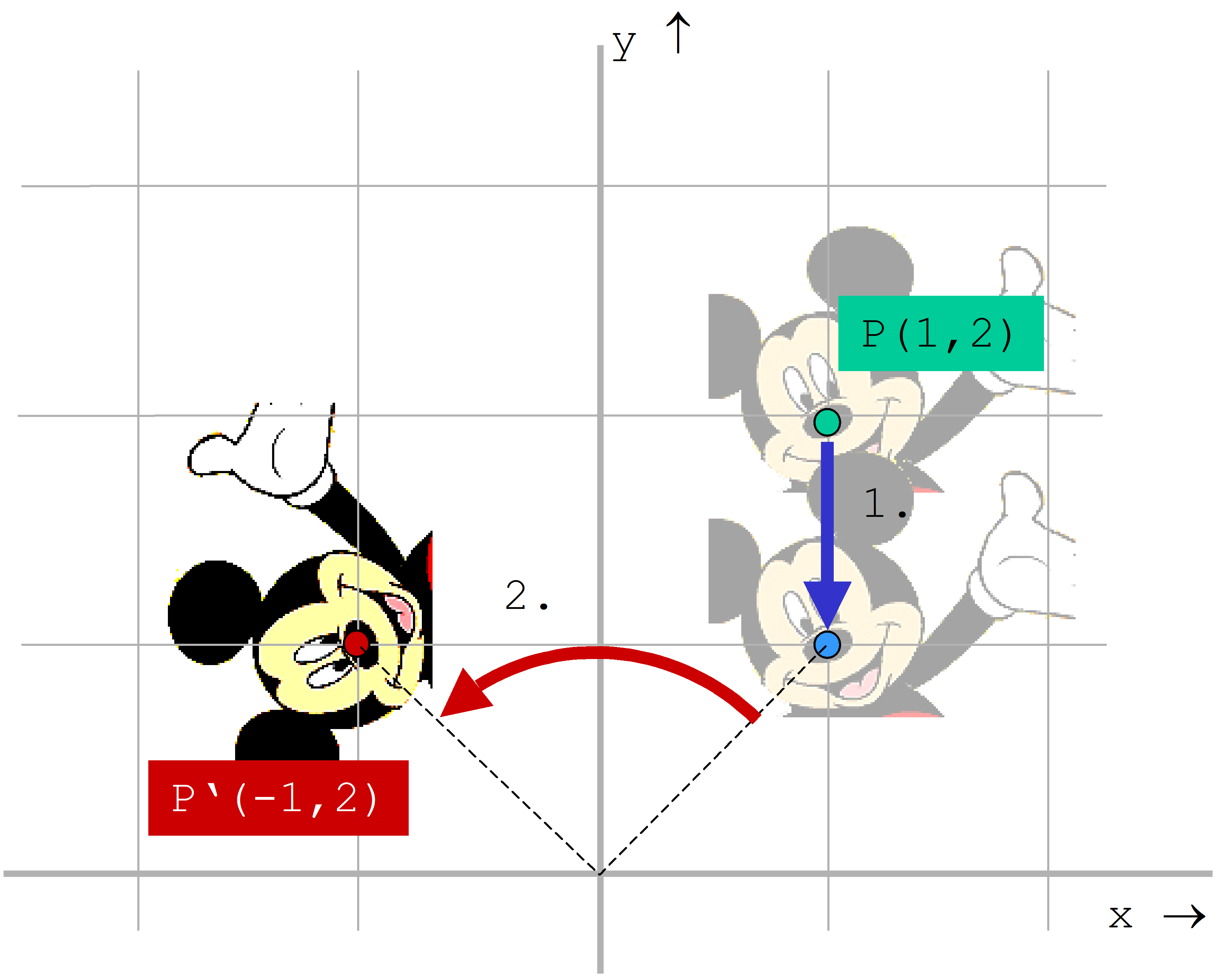
Beispiel 1:
Gegeben sei der Punkt P(1;2). Dieser sei zunächst um eine Einheit parallel zur y-Achse in Richtung Koordinatenursprung zu verschieben und anschließend um einen Winkel von 90° zu rotieren. Die Lösung sieht demnach so aus:
\(P' = R · T · P = \left( {\begin{array}{cc}0&{ - 1}&0\\1&0&0\\0&0&1\end{array} } \right) \cdot \left( {\begin{array}{cc}1&0&0\\0&1&{ - 1}\\0&0&1\end{array} } \right) \cdot \left( {\begin{array}{cc}x\\y\\1\end{array} } \right)\)
Bei der Aneinanderfügung der Faktoren ist immer die richtige Reihenfolge – von rechts nach links - zu beachten! Zunächst werden die beiden Transformationsmatrizen multipliziert:
\(P' = R · T · P = \left( {\begin{array}{cc}0&{ - 1}&1\\1&0&0\\0&0&1\end{array} } \right) \cdot \left( {\begin{array}{cc}x\\y\\1\end{array} } \right)\)
Mit x=1 und y=2 ergibt sich der transformierte Punkt zu
\(P' = R · T · P = \left( {\begin{array}{cc}0&{ - 1}&1\\1&0&0\\0&0&1\end{array} } \right) \cdot \left( {\begin{array}{cc}1\\2\\1\end{array} } \right) = \left( {\begin{array}{cc}{ - 1}\\1\\1\end{array} } \right)\)
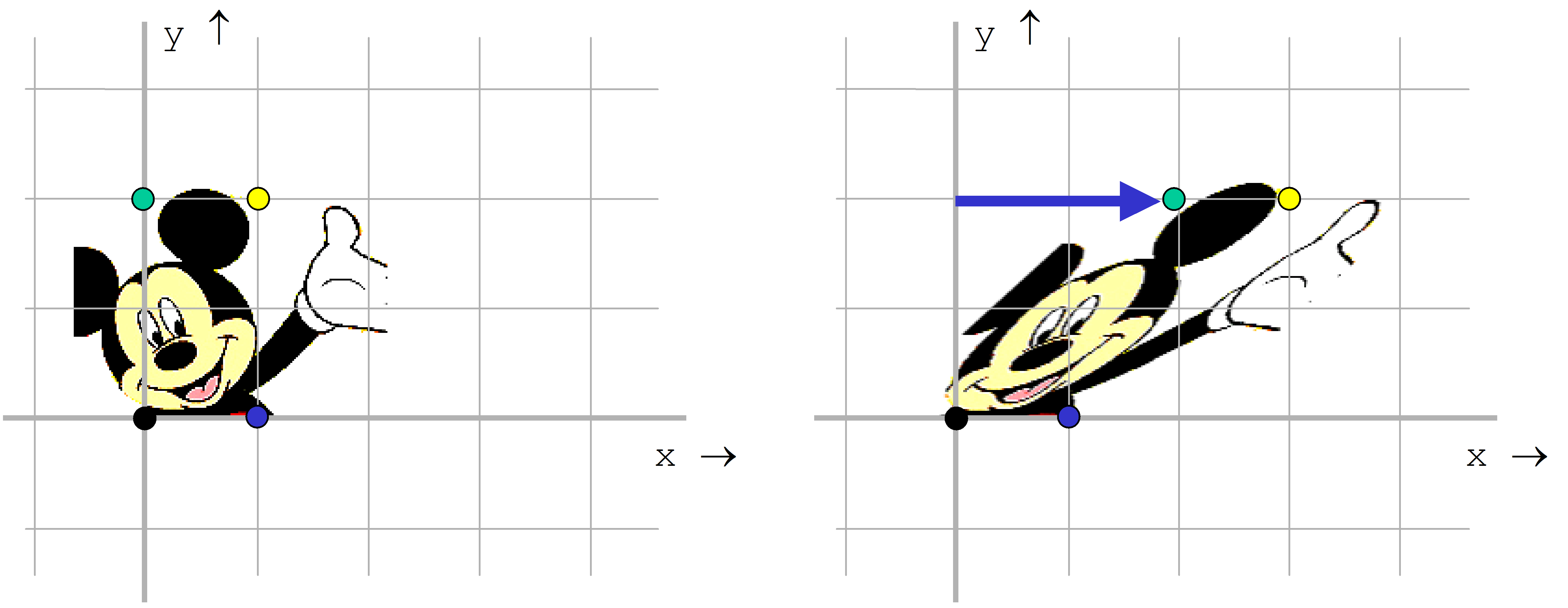
Beispiel 2:
Ein Rechteck, das durch die Punkte P1(0;0), P2(0;2), P3(1;2) und P4(1;0) gegeben ist, soll parallel der x-Achse um 45° geschert werden. Mit a=45° und b=0° werden ax=tan(45°)=1 und ay=tan(0)=0. Folglich gilt:
\( Sh = \left( {\begin{array}{cc}1&1&0\\0&1&0\\0&0&1\end{array} } \right) \)
Daraus ergeben sich die neuen Punkte:
\( P1' = Sh \cdot P1 = \left( {\begin{array}{cc}1&1&0\\0&1&0\\0&0&1\end{array} } \right) \cdot \left( {\begin{array}{cc}0\\0\\1\end{array} } \right) = \left( {\begin{array}{cc}0\\0\\1\end{array} } \right) \\ P2' = Sh \cdot P2 = \left( {\begin{array}{cc}1&1&0\\0&1&0\\0&0&1\end{array} } \right) \cdot \left( {\begin{array}{cc}0\\2\\1\end{array} } \right) = \left( {\begin{array}{cc}2\\2\\1\end{array} } \right) \)
\(P3' = Sh \cdot P3 = \left( {\begin{array}{cc}1&1&0\\0&1&0\\0&0&1\end{array} } \right) \cdot \left( {\begin{array}{cc}1\\2\\1\end{array} } \right) = \left( {\begin{array}{cc}3\\2\\1\end{array} } \right) \\ P4' = Sh \cdot P4 = \left( {\begin{array}{cc}1&1&0\\0&1&0\\0&0&1\end{array} } \right) \cdot \left( {\begin{array}{cc}1\\0\\1\end{array} } \right) = \left( {\begin{array}{cc}1\\0\\1\end{array} } \right)\)